Different KL Estimators and their correctness for Reinforcement Learning
Intro
Often times in Reinforcement Learning (and Machine learning in general), we would like to estimate the Kullback-Leibler (KL) divergence of our current policy with respect to a reference policy, and for many good reasons. For example in offline RL, we want reward-maximizing behavior without overoptimizing outside the data support (otherwise we run into OOD issues at test time). And in off-policy online RL, we want better sample efficiency by taking multiple gradient steps per batch, but we can’t stray too far, otherwise our policy gradient objectives are no longer valid. As for why KL specifically and not some other constraint? While we do use other ones like Wasserstein, the KL-regularization solution has a well-known closed form solution, and in general is pretty clean to work with. But getting KL exactly right in practice is harder than it looks!
KL Divergence
The KL divergence gives a quantifiable measure of how different two distributions are. It’s non-negative asymmetric. Given a reference policy \(\mu\) and the policy we are training, \(p_\theta\):
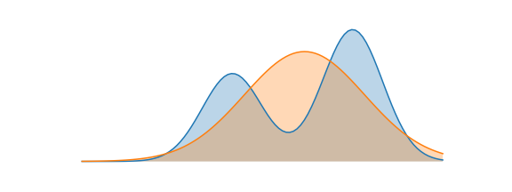
- Forward KL: \(D_{KL}(\mu \| p_\theta) = \mathbb{E}_{x \sim \mu}\left[\log\frac{\mu(x)}{p_\theta(x)}\right]\). Minimizing this moves mass from \(p_\theta\) to cover all modes of \(\mu\) — a.k.a. mode covering.
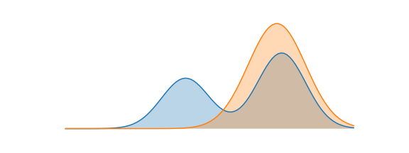
- Reverse KL: \(D_{KL}(p_\theta \| \mu) = \mathbb{E}_{x \sim p_\theta}\left[\log\frac{p_\theta(x)}{\mu(x)}\right]\). Minimizing this restricts \(p_\theta\) from placing mass anywhere \(\mu\) doesn’t — a.k.a. mode seeking.
In LLM RL, Offline RL, and most behavior regularization settings, reverse KL is typically used because we want to stay close to the reference rather than cover every mode.
When do we use KL Divergence in RL?
There are two main places KL estimates appear in RL training:
- As a detached reward bonus — subtracted from the reward signal, not differentiated through (e.g.
reward -= beta * kl.detach()) - As a differentiable loss term — directly backpropagated as a regularizer alongside the policy loss
Both the type of KL (forward vs. reverse) and how we use it change which estimator is correct. Mixing these up can lead a lot of sneaky bugs.
Off-policy vs on-policy
Where our training samples come from matters because forward and reverse KL have different expectations. If samples come from our current policy \(p_\theta\), we’re on-policy. If they come from something else (a fixed behavior policy, an older version of \(p_\theta\), human demos), we’re off-policy.
For off-policy scenarios, we can correct for the distribution mismatch using an importance weight \(\rho = \frac{p_\theta(x)}{\mu_\text{samp}(x)}\), where \(\mu_\text{samp}\) is wherever the samples came from. Note that in the on-policy case, \(\rho \equiv 1\) numerically — but as we’ll see, it still matters for gradients.
The three estimators
Why do we estimate KL rather than compute it exactly? Because taking expectations over all outputs of a large neural network is intractable. So in practice, we use Monte Carlo samples. The three main estimators in the literature (originally from Schulman [2]) are:
k1 = \(\log \frac{p_\theta(x)}{\mu(x)}\). This is the direct single-sample estimate of the reverse KL. It is clearly unbiased, but the downside is that individual samples can go negative even though true KL is non-negative, so relative variance can be high.
k2 = \(\frac{1}{2}\left(\log \frac{\mu(x)}{p_\theta(x)}\right)^2\). k2 is always non-negative, however it is biased (its expectation is not exactly the KL.) But near \(p_\theta \approx \mu\) the bias is actually quite small, and it shares the same second-order Taylor expansion as reverse KL around the identity. So you can think of it as a locally valid surrogate objective for the KL.
k3 = \(\frac{\mu(x)}{p_\theta(x)} - 1 - \log\left(\frac{\mu(x)}{p_\theta(x)}\right)\). k3 is also unbiased: the \(\frac{\mu}{p_\theta} - 1\) part has expectation 0, so k3 is k1 plus a zero-mean control variate that reduces variance. It is also always non-negative by Jensen’s inequality (since \(\log x \leq x - 1\)). Furthermore, when \(p_\theta\) and \(\mu\) are close, k3 typically has lower variance than k1. But if they diverge significantly the \(\frac{\mu}{p_\theta}\) ratio can blow up. This is why the Composer 2 tech report [3] decided to use k1 instead of k3.
| Unbiased for reverse KL? | Non-negative? | Variance (when policies are close) | |
|---|---|---|---|
| k1 | Yes | No | High |
| k2 | No (small near KL≈0) | Yes | Low |
| k3 | Yes | Yes | Low |
Gradients of the estimators
Before talking about which to use, let’s derive their (analytical) gradients, because being close in value doesn’t mean that the gradients are also close. Let \(s_\theta = \nabla_\theta \log p_\theta(x)\) denote the score function, and an important identity is the score function identity: \(\mathbb{E}_{p_\theta}[s_\theta] = 0\).
- \(\nabla_\theta k_1 = s_\theta\) (since \(k_1 = \log p_\theta - \log \mu\), and \(\mu\) doesn’t depend on \(\theta\))
- \(\nabla_\theta k_2 = -\left(\log \frac{\mu}{p_\theta}\right) s_\theta\). You can can verify this using chain rule.
- \(\nabla_\theta k_3 = \left(1 - \frac{\mu}{p_\theta}\right) s_\theta\). You can verify this by using chain rule and product rule on the two pieces.
And for reference, the true gradient of reverse KL (derived by differentiating \(\int p_\theta \log \frac{p_\theta}{\mu}\, dx\) via product rule + score identity) is:
\[\nabla_\theta D_{KL}(p_\theta \| \mu) = \mathbb{E}_{p_\theta}\!\left[s_\theta \cdot \log \frac{p_\theta}{\mu}\right] = \mathbb{E}_{p_\theta}[s_\theta \cdot k_1]\]Using as a differentiable loss term
When KL is backpropagated directly, we need its gradient expectation to equal \(\nabla_\theta D_{KL}(p_\theta \| \mu)\). This is where things get tricky…
Autodiff issues
The naive approach would just be to sample \(x \sim p_\theta\), compute \(k_i(x)\), call .backward(). This gives gradient expectation \(\mathbb{E}_{p_\theta}[\nabla_\theta k_i]\) — but this is NOT the same as \(\nabla_\theta \mathbb{E}_{p_\theta}[k_i]\), because the sampling distribution itself depends on \(\theta\), which autograd doesn’t account for. Now you may ask, why don’t we just use rsample()? While the reparameterization trick works for continuous gaussian policies, for something like an LLM w/ discrete tokens, you can’t really parameterize a categorical distribution as a function of \(\theta\) and noise \(\epsilon\). (you could try a gumbel-softmax, but then the gradient will be biased.)
The result:
-
k1 naively: \(\mathbb{E}_{p_\theta}[\nabla_\theta k_1] = \mathbb{E}_{p_\theta}[s_\theta] = \mathbf{0}\). The gradient is zero-meaned, which is incorrect, and furthermore doesn’t even include a \(\mu\) term, so it is not very useful as a regularizer. This is why something like
(curr_log_probs - ref_log_probs).mean()does nothing as a KL regularizer. -
k2 naively: \(\mathbb{E}_{p_\theta}[\nabla_\theta k_2] = \nabla_\theta D_{KL}(p_\theta \| \mu)\). Maybe surprisingly, k2 actually does work in the naive implementation because the chain rule fills in the missing score-function term correctly!
-
k3 naively: \(\mathbb{E}_{p_\theta}[\nabla_\theta k_3] = \nabla_\theta D_{KL}(\mu \| p_\theta)\). Interesingly, this is the forward KL gradient, which is the wrong direction for Reverse KL regularization! So if you naively backprop through k3 thinking you’re doing reverse KL, you’re actually minizing Forward KL.
The fix
Oftentimes in order to make auto-diff give us the correct gradients, we use a surrogate objective that isn’t technically correct, bu the gradients are! The fix here is to explicitly construct an additional term \(\rho = p_\theta(x) / \text{sg}(\mu(x))\), where sg is detaching the gradients to our reference policy. This will essentially force autograd to pick up the score-function path during auto-differentiation. Note in the on-policy case, \(\rho \equiv 1\) numerically — but \(\nabla_\theta \rho = s_\theta \neq 0\), which is exactly the term that we were missing in the naive scenario.
I won’t go into the derivations here, but now with \(\rho\) explicit, the gradient-correct options for reverse KL are:
| Loss form | Gradient expectation | Notes |
|---|---|---|
| \(\rho \cdot k_1\) | \(\nabla_\theta D_{KL}(p_\theta | \mu)\) Yes | Higher variance |
| \(\text{sg}(\rho) \cdot k_2\) | \(\nabla_\theta D_{KL}(p_\theta | \mu)\) Yes | Low variance |
| \(\rho \cdot k_3\) | \(\nabla_\theta D_{KL}(p_\theta | \mu)\) Yes | Low variance |
An interesting note is that \(\text{sg}(\rho) \cdot k_2\) and \(\rho \cdot k_3\) actually produce sample-wise identical gradients (both equal \(\rho s_\theta k_1\)). For the full derivations, see Wang [4].
Quick reference for loss term:
| Setting | Recommended | Reasoning |
|---|---|---|
| On-policy | k2 (naive backprop) | Expectation is already over \(p_\theta\), so \(\nabla k2\) lands on the correct gradient |
| Off-policy | \(\text{sg}(\rho) \cdot k2\) or \(\rho \cdot k3\) | Samples come from \(\mu_\text{samp} \neq p_\theta\); \(\rho\) re-weights to \(p_\theta\) |
The reason k2 is special on-policy: \(\mathbb{E}_{p_\theta}[\nabla_\theta k2] = \mathbb{E}_{p_\theta}[k1 \cdot s_\theta]\), which is exactly the reverse KL gradient. Off-policy, that expectation is over the wrong distribution, so we use sg\((\rho)\) as an IS weight to correct it.
Using KL as a detached reward bonus
Here’s where the most common mistake happens. Since k1 and k3 are both unbiased value estimators for reverse KL, you might think either is fine for reward shaping. But this is actually incorrect.
The reason is that when KL is a detached reward bonus (reward -= beta * kl.detach()), the KL term only influences training through the policy gradient. So for this to be an unbiased estimate of the true KL-regularized objective, we need the policy gradients to align:
-
k1: \(\mathbb{E}[s_\theta \cdot k_1] = \nabla_\theta D_{KL}(p_\theta \| \mu)\). So this is correct!
-
k3: \(\mathbb{E}[s_\theta \cdot k_3] = -\nabla_\theta D_{KL}(\mu \| p_\theta) + \nabla_\theta D_{KL}(p_\theta \| \mu)\). Note that the first term is adding a forward KL bias term! So despite being value-unbiased and lower variance, using k3 in reward shaping actually makes it a biased estimator
-
k2: this is also similarly biased in the policy gradient term.
So TLDR is that for reward shaping, we really only want to use k1. The lower variance of k3 doesn’t matter here because it changes what you’re actually optimizing.
Summary
To wrap things up, the choice of which estimator to use mainly depends on 3 questions: (1) are samples on-policy or off-policy, (2) is KL a differentiable loss or a detached reward bonus, and (3) are you constructing \(\rho\) explicitly?
The key insight from Wang [4] and Tang & Munos [5] is that value unbiasedness \(\neq\) gradient correctness. For example k3 looks great as a value estimator because it’s value is unbiased but it actually breaks in naive loss backprop (giving forward KL) and reward shaping (adding forward KL bias). On the other hand, k2 is biased as a value estimator but is the only estimator that actuallys works (albeit accidentally)in the naive on-policy loss case.
| Use case | Correct choice | Wrong choice |
|---|---|---|
| Detached reward bonus | \(k1\) | \(k3\) (value-unbiased but gradient-biased!) |
| Loss term, naive on-policy | \(k2\) | \(k1\) (zero gradient), \(k3\) (forward KL!) |
| Loss term, explicit \(\rho\) or off-policy | \(\text{sg}(\rho) \cdot \text{k2}\) or \(\rho \cdot \text{k3}\) | \(\rho \cdot \text{k2}\) (\(\rho\) kept in grad) |
References
- Dibya Ghosh. KL Divergence for Machine Learning. dibyaghosh.com/blog, 2023.
- John Schulman. Approximating KL Divergence. joschu.net/blog, 2020.
- Cursor. Composer 2 Technical Report. cursor.com/resources/Composer2.pdf, 2025.
- Xihuai Wang. Choosing KL Estimators in RL: From Value Unbiasedness to Gradient Correctness. xihuai18.github.io, 2025.
- Yunhao Tang and Rémi Munos. On a few pitfalls in KL divergence gradient estimation for RL. arXiv:2506.09477, 2025.